Download as Python script

Download as Jupyter notebook

Download as PDF document

---

Multifunction radar parametric study

This tutorial demonstrates how to conduct a parametric study on a multifunction radar system using PySTK. It is inspired by this tutorial.

What are important parameters in a multifunction radar?

A multifunction radar models multiple radar beams working together at the same location. Each beam has its own specifications and constraints. Some important settings include beam gain, goal signal to noise ratio (SNR), and maximum number of pulses integrated.

Beam gain measures how the antenna for a beam concentrates power in a certain direction. It is related to both efficiency and directivity. The optimal gain value depends on how an antenna is being used. The best choice for hitting a receiver far away is a high-gain value, as the signal has to travel over a large distance, so it needs to be intensified and pointed directly at the target. If the signal must be received evenly over a broad area, however, lower gain is more appropriate.

Signal to noise ratio is a measure that compares the level of a desired signal to the level of noise. To increase SNR, radar systems often use multiple pulse integration which is the process of summing multiple transmit pulses to improve detection. When a target is located within the radar beam during a single scan, it may reflect several pulses. By adding the returns from all pulses returned by a given target during a single scan, the radar sensitivity SNR can be increased. With STK’s Goal SNR setting, STK integrates up to the maximum pulse number to achieve the desired signal-to-noise ratio.

The effectiveness of a certain radar configuration can be measured by the probability of detection for a designated target, which is always between 0 and 1. The probability of detection is a function of the per pulse signal to noise ratio (SNR), the number of pulses integrated, the probability of false alarm and the radar cross section (RCS) fluctuation type. STK reports the probability of detection based off of a single pulse (S/T Pdet1), and over all integrated pulses (S/T Integrated PDet).

Problem statement

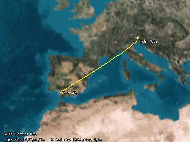
An aircraft leaves an airbase in Spain and flies to an airbase in Italy. The aircraft has a constant radar cross section value of \(20\) dBsm. A radar site located at an Italian airbase employs a multifunction radar which tracks the inbound aircraft. Terrain is accounted for analytically in the vicinity of the radar site. An integrated PDet value of 0.8 to 1.0 is required to track the aircraft with certainty. Determine how beam gain, signal to noise ratio, and pulse integration affect the multifunction radar’s ability to track the aircraft.

Conduct parametric studies varying:

• Gain from \(20\) dB to \(40\) dB in \(2\) dB increments.

• Goal SNR from \(10\) dB to \(22\) dB in \(1\) dB increments.

• Maximum number of pulses from \(1\) to \(200\) in increments of \(10\).

• Gain from \(20\) to \(40\) dB in increments of \(5\) dB, and goal SNR from \(10\) to \(20\) dB in increments of \(2\) dB at the same time.

Launch a new STK instance

Start by launching a new STK instance. In this example, STKEngine is used.

from ansys.stk.core.stkengine import STKEngine


stk = STKEngine.start_application(no_graphics=False)

Load the starter scenario

The STK scenario used in this tutorial is included with the STK installation as a VDF file. To open the scenario, first access the STK Root object:

root = stk.new_object_root()

Then, load the VDF from the path:

import pathlib


install_dir = pathlib.Path(root.execute_command("GetDirectory / STKHome")[0])
scenario_filepath = str(
    install_dir
    / "Data"
    / "Resources"
    / "stktraining"
    / "VDFs"
    / "MFR_Analyzer_Starter.vdf"
)
root.load_vdf(scenario_filepath, "")

Next, get the current scenario using the root object:

scenario = root.current_scenario

Once the scenario is loaded, it is possible to show a 3D graphics window and view the aircraft’s route by running:

from ansys.stk.core.stkengine.experimental.jupyterwidgets import GlobeWidget


globe_plotter = GlobeWidget(root, 640, 480)
globe_plotter.camera.position = [7934, 1684, 7025]
globe_plotter.show()

Compute initial radar access

The radar has a single beam, identified as the TargetTransport beam, which targets the aircraft with a gain value of \(30\) dB. The beam uses a waveform strategy similar to the medium range rectangular strategy.

To determine how well the radar detects the aircraft with its initial settings, first get the radar object using the STK root object and the radar’s path:

mfr = root.get_object_from_path("/Place/Radar_Site/Radar/MFR")

Then, get the aircraft object:

aircraft = root.get_object_from_path("/Aircraft/Aircraft/")

Create an access between the radar and the aircraft and compute the access:

access = mfr.get_access_to_object(aircraft)
access.compute_access()

Any beams that are part of a radar become a data provider group under that radar’s Radar Multifunction provider. To get the data for the TargetTransport beam, first select the access’s Radar Multifunction provider, then select the TargetTransport group:

target_transport_provider = access.data_providers.item(
    "Radar Multifunction"
).group.item("TargetTransport")

Determine the start and end times of the access:

access_start, access_stop = access.computed_access_interval_times.get_interval(0)
f"The access starts at {access_start} and ends at {access_stop}."

'The access starts at 1 Apr 2020 14:23:46.580 and ends at 1 Apr 2020 15:14:31.481.'

Get the S/T integrated SNR, S/T Integrated PDet, and S/T Pulses Integrated over time during the access, using a 10 second time step, and convert the data to a pandas dataframe:

elements = [
    "Time",
    "S/T Integrated SNR",
    "S/T Integrated PDet",
    "S/T Pulses Integrated",
]
access_df = target_transport_provider.execute_elements(
    access_start, access_stop, 10, elements
).data_sets.to_pandas_dataframe()

Display the first five rows of the data:

access_df.head(5)

	s/t integrated pdet	s/t integrated snr	s/t pulses integrated	time
0	0.00010844276338245851	-3.645526969990879	512	1 Apr 2020 14:23:46.580445000
1	0.00010856329690121817	-3.5843944131843024	512	1 Apr 2020 14:23:56.000000000
2	0.00010869355863454479	-3.5193122573711015	512	1 Apr 2020 14:24:06.000000000
3	0.00010882623823921913	-3.4540408523313646	512	1 Apr 2020 14:24:16.000000000
4	0.00010896138561382438	-3.3885790523754404	512	1 Apr 2020 14:24:26.000000000

Then, determine during how many time steps the aircraft can be tracked with at least 80% confidence:

access_df["s/t integrated pdet"] = access_df["s/t integrated pdet"].astype(float)
f"The aircraft can be tracked with certainty during {len(access_df[access_df['s/t integrated pdet'] >= 0.8])} time steps, out of {len(access_df)} total."

'The aircraft can be tracked with certainty during 60 time steps, out of 306 total.'

Determine the first time at which the aircraft can be tracked with certainty:

import pandas as pd


# convert and sort time data
access_df["time"] = pd.to_datetime(access_df["time"])
access_df = access_df.sort_values(by="time", ascending=True)

first_time = access_df[access_df["s/t integrated pdet"] >= 0.8].iloc[0]["time"]
f"The first time that the S/T Integrated PDet is at or above 0.8 is {first_time}."

'The first time that the S/T Integrated PDet is at or above 0.8 is 2020-04-01 15:04:46.'

Then, determine how long the radar tracks the aircraft:

time_delta = (
    access_df[access_df["s/t integrated pdet"] >= 0.8].iloc[-1]["time"]
    - (access_df[access_df["s/t integrated pdet"] >= 0.8].iloc[0]["time"])
)
f"The radar tracks the aircraft for approximately {(time_delta.total_seconds() / 60):.2f} minutes."

'The radar tracks the aircraft for approximately 9.76 minutes.'

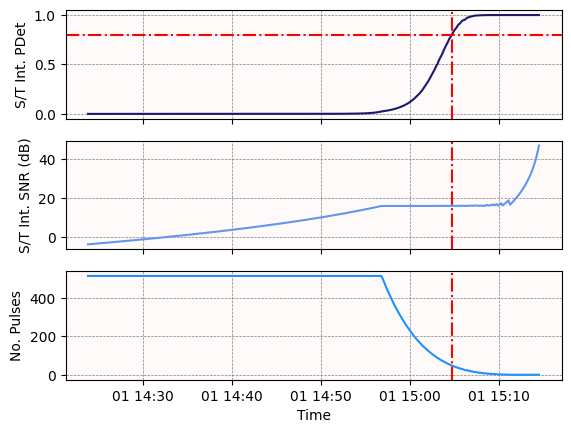
Next, graph the S/T Integrated SNR, S/T Pulses Integrated, and S/T Integrated PDet throughout the access. As the S/T Integrated PDet improves, S/T Integrated SNR increases and S/T Pulses Integrated decreases.

import matplotlib.pyplot as plt


# data conversions
access_df["s/t integrated snr"] = access_df["s/t integrated snr"].astype(float)
access_df["s/t pulses integrated"] = access_df["s/t pulses integrated"].astype(float)

# create plot with shared x-axis
fig, axes = plt.subplots(3, 1, sharex=True)

# plot integrated PDet, integrated SNR, and pulses integrated against time on 3 different plots
axes[0].plot(
    access_df["time"],
    access_df["s/t integrated pdet"],
    linestyle="-",
    color="midnightblue",
)
axes[1].plot(
    access_df["time"],
    access_df["s/t integrated snr"],
    linestyle="-",
    color="cornflowerblue",
)
axes[2].plot(
    access_df["time"],
    access_df["s/t pulses integrated"],
    linestyle="-",
    color="dodgerblue",
)

# format axes
for ax in axes:
    ax.grid(True, color="gray", linestyle="--", linewidth=0.5)
    # add line corresponding to first time aircraft can be detected with certainty
    ax.axvline(first_time, color="red", linestyle="-.")
    ax.set_facecolor("snow")

axes[0].set_ylabel("S/T Int. PDet")
axes[1].set_ylabel("S/T Int. SNR (dB)")
axes[2].set_ylabel("No. Pulses")
plt.xlabel("Time")

# add line indicating pdet that corresponds to detection with certainty
axes[0].axhline(y=0.8, color="r", linestyle="-.")

plt.show()

Determine the impacts of gain

Antenna gain indicates how strong a signal an antenna can send or receive in a specified direction. Conduct a trade study to determine affect of gain on S/T Integrated PDet.

First, get the multifunction radar system’s TargetTransport beam:

target_transport = mfr.model_component_linking.component.antenna_beams.item(0)

The current gain is \(30\) dB. Vary the gain from \(20\) dB to \(40\) dB in \(2\) dB increments by setting the beam’s gain property. For each gain value, recompute the access between the radar and the aircraft, get the S/T Integrated PDet over the access interval, and then compute the mean PDet:

gain_values = list(range(20, 42, 2))
mean_pdets = []

for gain in gain_values:
    target_transport.gain = gain
    access.compute_access()
    pdet_df = (
        access.data_providers.item("Radar Multifunction")
        .group.item("TargetTransport")
        .execute_elements(access_start, access_stop, 10, ["S/T Integrated PDet"])
        .data_sets.to_pandas_dataframe()
    )
    mean_pdets.append(pdet_df.loc[:, "s/t integrated pdet"].mean())

Visualize the data as a line chart to determine how varying gain values affect PDet:

plt.plot(gain_values, mean_pdets, color="dodgerblue")
plt.grid(True, color="gray", linestyle="--", linewidth=0.5)
plt.xlabel("Gain (dB)")
plt.ylabel("S/T Integrated PDet")
plt.gca().set_facecolor("snow")
plt.show()

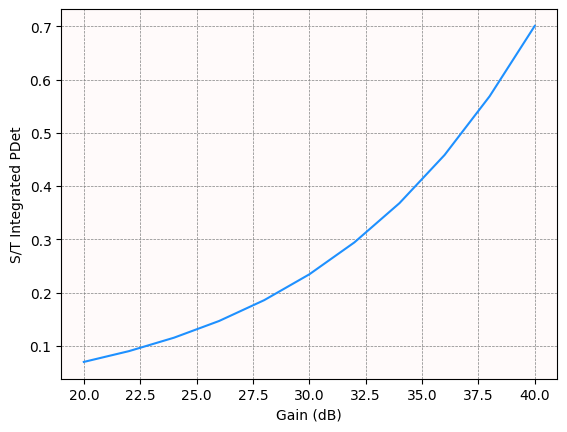
The mean S/T Integrated PDet has a slight increase from a gain of \(20\) dB through \(30\) dB. However, from \(30\) dB through \(40\) dB there is a steeper climb.

Before conducting another trade study, reset the antenna gain to \(30\) dB:

target_transport.gain = 30

Determine the impacts of goal SNR

Goal SNR is an integration analysis based on the desired signal-to-noise ratio. Conduct a second trade study to determine how varying goal SNR affects S/T Integrated PDet.

First, to set the goal SNR, get the radar model’s detection processing settings:

detection_processing = mfr.model_component_linking.component.detection_processing

Then, get the pulse integration settings. Pulse integration is set to use goal SNR, so the pulse_integration property returns a RadarPulseIntegrationGoalSNR object, through which it is possible to specify the goal SNR.

from ansys.stk.core.stkobjects import RadarPulseIntegrationGoalSNR


pulse_integration = RadarPulseIntegrationGoalSNR(detection_processing.pulse_integration)

The current goal SNR is \(16\) dB. Vary the goal SNR from \(10\) dB to \(22\) dB in \(1\) dB increments by setting the snr property on this object. For each SNR value, recompute the access between the radar and the aircraft, get the S/T Integrated PDet over the access interval, and then compute the mean PDet:

mean_pdets = []
snr_values = list(range(10, 23))

for snr in snr_values:
    pulse_integration.snr = snr
    access.compute_access()
    pdet_df = (
        access.data_providers.item("Radar Multifunction")
        .group.item("TargetTransport")
        .execute_elements(access_start, access_stop, 10, ["S/T Integrated PDet"])
        .data_sets.to_pandas_dataframe()
    )
    mean_pdets.append(pdet_df.loc[:, "s/t integrated pdet"].mean())

Visualize the data as a line chart to determine how varying goal SNR values affect PDet:

plt.plot(snr_values, mean_pdets, color="dodgerblue")
plt.grid(True, color="gray", linestyle="--", linewidth=0.5)
plt.xlabel("Goal SNR (dB)")
plt.ylabel("S/T Integrated PDet")
plt.gca().set_facecolor("snow")
plt.show()

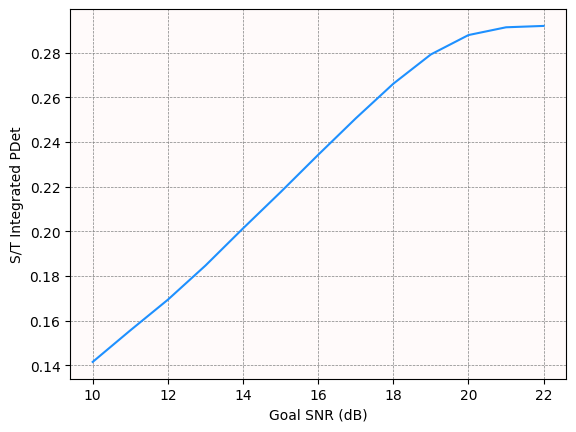
There is a steady increase in mean S/T Integrated PDet until the goal SNR reaches \(20\) dB.

Before continuing to the next trade study, reset the goal SNR to \(16\) dB:

pulse_integration.snr = 16

Determine the impact of the number of maximum pulses

Conduct a trade study to determine how varying the maximum number of pulses integrated affects S/T Integrated PDet.

The maximum number of pulses is \(512\). Vary the maximum number from \(1\) to \(200\) in increments of \(10\) by setting the maximum_pulses property on the pulse integration settings object. For each value, recompute the access between the radar and the aircraft, get the S/T Integrated PDet over the access interval, and then compute the mean PDet:

max_pulse_values = list(range(1, 210, 10))
mean_pdets = []

for max_pulse_number in max_pulse_values:
    pulse_integration.maximum_pulses = max_pulse_number
    access.compute_access()
    pdet_df = (
        access.data_providers.item("Radar Multifunction")
        .group.item("TargetTransport")
        .execute_elements(access_start, access_stop, 10, ["S/T Integrated PDet"])
        .data_sets.to_pandas_dataframe()
    )
    mean_pdets.append(pdet_df.loc[:, "s/t integrated pdet"].mean())

Visualize the data as a line chart to determine how varying maximum pulse number values affect PDet:

plt.plot(max_pulse_values, mean_pdets, color="dodgerblue")
plt.grid(True, color="gray", linestyle="--", linewidth=0.5)
plt.xlabel("Maximum Number of Pulses")
plt.ylabel("S/T Integrated PDet")
plt.gca().set_facecolor("snow")
plt.show()

The mean integrated probability of detection has a sharp rise until 50 pulses integrated, after which it begins to level off.

Before continuing, reset the maximum number of pulses to the default of \(512\):

pulse_integration.maximum_pulses = 512

Determine the impact of varying gain and goal SNR at the same time

Finally, determine how varying gain and goal SNR at the same time impact the probability of detection. Vary the gain from \(20\) to \(40\) dB in increments of \(5\) dB, and vary the goal SNR from \(10\) to \(20\) dB in increments of \(2\) dB. For each combination of gain and goal SNR values, recompute the access between the radar and the aircraft, get the S/T Integrated PDet over the access interval, and then compute the mean PDet:

snrs = list(range(10, 22, 2))
gains = list(range(20, 45, 5))
mean_pdets = []
for i in range(len(snrs)):
    snr = snrs[i]
    mean_pdets.append([])
    pulse_integration.snr = snr
    for gain in gains:
        target_transport.gain = gain
        access.compute_access()
        pdet_df = (
            access.data_providers.item("Radar Multifunction")
            .group.item("TargetTransport")
            .execute_elements(access_start, access_stop, 10, ["S/T Integrated PDet"])
            .data_sets.to_pandas_dataframe()
        )
        mean_pdets[i].append(pdet_df.loc[:, "s/t integrated pdet"].mean())

Then, visualize the data using a carpet plot, which is a means of displaying data dependent on two variables in a format that makes interpretation easier than normal multiple curve plots. A carpet plot can be used to help with interpreting a multi-dimensional parametric study.

import plotly.graph_objects as go


# create figure
fig = go.Figure()

# add carpet with gain and goal SNR values as independent variables, and PDet as the dependent variable
fig.add_trace(
    go.Carpet(
        a=gains,
        b=snrs,
        y=mean_pdets,
        name="pdet_plot",
        aaxis=dict(
            smoothing=1,
            minorgridcount=9,
            minorgridwidth=0.6,
            minorgridcolor="white",
            gridcolor="white",
            color="black",
            title="Gain (dB)",
            type="linear",
        ),
        baxis=dict(
            smoothing=1,
            minorgridcount=9,
            minorgridwidth=0.6,
            gridcolor="white",
            minorgridcolor="white",
            color="black",
            title="SNR (dB)",
            type="linear",
        ),
    )
)

# configure layout and title
fig.update_layout(
    width=1200, height=600, title_text="S/T Integrated PDet vs. Goal SNR and Gain"
)

# add contours coloring plot based on PDet value
fig.add_trace(
    go.Contourcarpet(
        a=gains,
        b=snrs,
        z=mean_pdets,
        autocontour=False,
        contours=dict(start=0, end=0.85, size=0.05),
        line=dict(width=2, smoothing=0),
        colorbar=dict(len=0.4, y=0.25, title=dict(text="S/T Integrated PDet")),
    )
)
fig.show(renderer="notebook")

Then, use the plot to determine what the predicted average PDet value would be for a gain of \(36\) dB and a goal SNR of \(16\) dB. To do so, add lines to the plot showing where these values intersect. The intersection of these lines represents an interpolation of the outcome for these parameters.

import numpy as np


constant_gain = 36
constant_snr = 16
num_gain_points = len(gains)
num_snr_points = len(snrs)

# add line at constant value of 36 dB gain
fig.add_trace(
    go.Scattercarpet(
        a=np.full(num_snr_points, constant_gain),
        b=snrs,
        mode="lines",
        line=dict(shape="spline", smoothing=1, color="black", width=3),
        showlegend=False,
    )
)

# add line at constant value of 16 dB SNR
fig.add_trace(
    go.Scattercarpet(
        a=gains,
        b=np.full(num_gain_points, constant_snr),
        mode="lines",
        line=dict(shape="spline", smoothing=1, color="black", width=3),
        showlegend=False,
    )
)

# add point corresponding to 36 dB gain and 16 dB SNR
fig.add_trace(
    go.Scattercarpet(
        a=[36],
        b=[16],
        line=dict(
            shape="spline",
            smoothing=1,
            color="black",
        ),
        marker=dict(
            size=15, color="white", symbol="circle", line=dict(color="black", width=2)
        ),
        showlegend=False,
    )
)

fig.show(renderer="notebook")

A gain of \(36\) dB and goal SNR of \(16\) dB are predicted to give an integrated PDet of approximately 0.41.

Then, use STK to calculate the actual PDet produced by a gain of \(36\) dB and goal SNR of \(16\) dB:

pulse_integration.snr = 16
target_transport.gain = 36
access.compute_access()
pdet_df = (
    access.data_providers.item("Radar Multifunction")
    .group.item("TargetTransport")
    .execute_elements(access_start, access_stop, 10, ["S/T Integrated PDet"])
    .data_sets.to_pandas_dataframe()
)
pdet = pdet_df.loc[:, "s/t integrated pdet"].mean().item()
f"The PDet is {pdet:.2f}."

'The PDet is 0.46.'

So, the PDet predicted using the carpet plot is approximately 0.05 less than the actual PDet.

Finally, determine the gain and SNR values that produce the highest and lowest PDets:

min_linear_index = np.argmin(mean_pdets)
min_coords = np.unravel_index(min_linear_index, np.shape(mean_pdets))
min_snr_index = min_coords[0]
min_gain_index = min_coords[1]
print(
    f"An SNR of {snrs[min_snr_index]} dB and a gain of {gains[min_gain_index]} dB produce the minimum PDet of {mean_pdets[min_snr_index][min_gain_index]:.2f}."
)
max_linear_index = np.argmax(mean_pdets)
max_coords = np.unravel_index(max_linear_index, np.shape(mean_pdets))
max_snr_index = max_coords[0]
max_gain_index = max_coords[1]
print(
    f"An SNR of {snrs[max_snr_index]} dB and a gain of {gains[max_gain_index]} dB produce the maximum PDet of {mean_pdets[max_snr_index][max_gain_index]:.2f}."
)

An SNR of 10 dB and a gain of 20 dB produce the minimum PDet of 0.04.
An SNR of 20 dB and a gain of 40 dB produce the maximum PDet of 0.85.