Download as Python script

Download as Jupyter notebook

Download as PDF document

---

Sensors and access

This tutorial demonstrates how to use different types of sensors to analyze access using Python and PySTK. It is inspired by this training.

What are sensors?

Sensor objects model the field-of-view and other properties of sensing devices attached to other STK objects. There are a large variety of sensor types that can be modeled in STK, including electro-optical and infrared sensors, parabolic antennas, push broom sensors, star trackers, and radars. Sensors can be customized in many ways, including by designating the properties of a sensor’s field-of-view. Additionally, sensors can behave in different ways. Sensors can be fixed to point in the same direction as their parent object’s reference frame, targeted to track other objects, or spinning to model instruments that spin, scan, or sweep over time. STK also allows the application of an azimuth-elevation mask to a sensor, and the consideration of this mask during calculations. A refraction model to constrain an atmosphere-based sensor’s line of sight and elevation angles can be modeled. It is also possible to customize the resolution of the sensor in terms of focus and image quality. Finally, many access constraints can be declared, including elevation, line of sight, sun, and temporal, on sensors to describe in what ways they can see other objects.

Problem statement

An air traffic control center is located in the Western United States between New Mexico and Wyoming. This area sees air traffic from a nearby airport, with the traffic flying between Cheyenne, Wyoming (latitude \(41.1400^\circ\), longitude \(-104.8202^\circ\)) and Raton, New Mexico (latitude \(36.9034^\circ\), longitude \(-104.4392^\circ\)). The center uses a radar system to track aircraft flying through the airport’s control zone. The center is located at a latitude of \(38.8006^\circ\) and a longitude of \(-104.6784^\circ\). The radar’s antenna is \(50\) ft (\(0.01524\) km) above ground. The center has two sensors: one fixed sensor with a field of view constrained by a range of \(150\) km, and one sweeping radar. The fixed sensor has a simple conic pattern with a cone half angle of \(90^\circ\). The sweeping radar has a rectangular pattern with a \(5^\circ\) vertical half angle and a \(35^\circ\) horizontal half angle. Determine how well these sensors are able to view an aircraft flying between Cheyenne and Raton.

Additionally, determine if a low earth orbit (LEO) satellite can take pictures of a ground site in Raton, and if it can take pictures of an aircraft as it flies between Cheyenne and Raton. The satellite flies in a low-earth circular orbit, with an inclination of \(60^\circ\), an altitude of \(800\) km, and a RAAN of \(20^\circ\). The satellite has two sensors: one fixed sensor with a simple conic pattern and a cone half angle of \(45^\circ\), and one sensor that is targeted towards Raton. The targeted sensor has a simple conic pattern with a cone half angle of \(5^\circ\). Determine if either of the satellite’s sensors can take pictures of Raton and the aircraft during the scenario period.

All sensors in the problem have angular resolutions of \(1^\circ\).

Launch a new STK instance

Start by launching a new STK instance. In this example, STKEngine is used.

from ansys.stk.core.stkengine import STKEngine


stk = STKEngine.start_application(no_graphics=False)
print(f"Using {stk.version}")

Using STK Engine v13.1.0

Create a new scenario

Create an STK scenario using the STK Root object:

root = stk.new_object_root()
root.new_scenario("SensorDesign")

Once the scenario is created, show a 3D graphics window by running:

from ansys.stk.core.experimental.jupyterwidgets import GlobeWidget


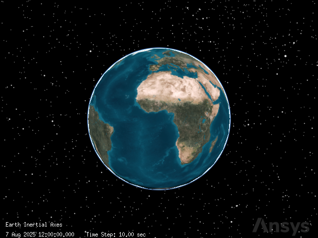
globe_plotter = GlobeWidget(root, 640, 480)
globe_plotter.show()

It is also possible to show a 2D graphics window by running:

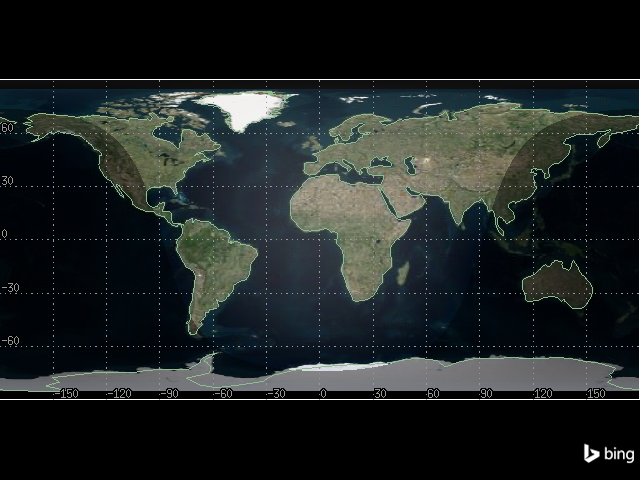
from ansys.stk.core.experimental.jupyterwidgets import MapWidget


map_plotter = MapWidget(root, 640, 480)
map_plotter.show()

Set the scenario time period

Using the newly created scenario, set the start and stop times. Rewind the scenario so that the graphics match the start and stop times of the scenario:

scenario = root.current_scenario
scenario.set_time_period("1 Jul 2016 16:00:00.000", "2 Jul 2016 16:00:00.000")
root.rewind()

Add the air traffic control center

The air traffic control center’s site is modeled with a place object. The radar site is located at a latitude of \(38.8006^\circ\) and a longitude of \(-104.6784^\circ\). The radar’s antenna is \(50\) ft (\(0.01524\) km) above the ground.

First, insert a place object to represent the airport’s radar site:

from ansys.stk.core.stkobjects import STKObjectType


radar_site = scenario.children.new(STKObjectType.PLACE, "RadarSite")

Then, set the radar site’s position using geodetic coordinates. Provide the latitude, longitude, and altitude corresponding to the radar’s antenna:

radar_site.position.assign_geodetic(38.8006, -104.6784, 0.01524)

Add relevant locations

Two places of interest in the vicinity of the radar site are Cheyenne, Wyoming, and Raton, New Mexico.

First, add a place object to represent Cheyenne:

cheyenne = scenario.children.new(STKObjectType.PLACE, "Cheyenne")

Cheyenne is located at a latitude of \(41.1400^\circ\) and a longitude of \(-104.8202^\circ\). Set the place’s location to match Cheyenne’s:

cheyenne.position.assign_geodetic(41.1400, -104.8202, 0)

Then, add a place object to represent Raton:

raton = scenario.children.new(STKObjectType.PLACE, "Raton")

Raton is located at a latitude of \(36.9034^\circ\) and a longitude of \(-104.4392^\circ\). Set the place’s location to match Raton’s:

raton.position.assign_geodetic(36.9034, -104.4392, 0)

Add an aircraft

To determine how well the radar site can view aircraft flying between Cheyenne and Raton, introduce a test aircraft flying between the cities to use in access calculations.

First, insert an aircraft:

aircraft = scenario.children.new(STKObjectType.AIRCRAFT, "Aircraft")

Because the aircraft’s route is defined by a set of waypoints, the aircraft’s flight is modeled with a Great Arc propagator. Set the aircraft’s propagator to the Great Arc propagator:

from ansys.stk.core.stkobjects import PropagatorType


aircraft.set_route_type(PropagatorType.GREAT_ARC)

The aircraft flies between Cheyenne and Raton, so the propagator’s route must include waypoints for both locations.

First, add a waypoint to the aircraft’s route to represent Cheyenne:

cheyenne_waypoint = aircraft.route.waypoints.add()

Set the waypoint’s location to match Cheyenne’s:

cheyenne_waypoint.latitude = 41.1400
cheyenne_waypoint.longitude = -104.8202

Then, add a waypoint to the route representing Raton:

raton_waypoint = aircraft.route.waypoints.add()

Set the waypoint’s location to match Raton’s:

raton_waypoint.latitude = 36.9034
raton_waypoint.longitude = -104.4392

Then, propagate the aircraft’s route:

aircraft.route.propagate()

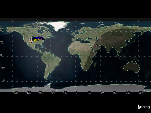
The 2D graphics window now shows the aircraft’s route, as well as both cities and the radar site:

map_plotter.camera.position = [6110, 34540, 0.0]
map_plotter.show()

Add a satellite

An imaging satellite flies in a low-earth circular orbit, with an inclination of \(60^\circ\), an altitude of \(800\) km, and a RAAN of \(20^\circ\). Determine if this satellite can view a site of interest at Raton.

First, insert a satellite:

satellite = scenario.children.new(STKObjectType.SATELLITE, "ImageSat")

Set the satellite’s propagator to J4Pertubation:

from ansys.stk.core.stkobjects import PropagatorType


satellite.set_propagator_type(PropagatorType.J4_PERTURBATION)
propagator = satellite.propagator

Set the orbit’s coordinate type to classical:

from ansys.stk.core.stkutil import OrbitStateType


orbit = propagator.initial_state.representation.convert_to(OrbitStateType.CLASSICAL)

Use the returned IOrbitStateClassical object to set the size_shape_type property. This property designates which pair of elements describe the orbit. Set the size_shape_type to Semimajor Axis and Eccentricity:

from ansys.stk.core.stkobjects import ClassicalSizeShape


orbit.size_shape_type = ClassicalSizeShape.SEMIMAJOR_AXIS

Set the orbit’s semimajor axis to \(7178.14\) km and it’s eccentricity to \(0\):

orbit.size_shape.semi_major_axis = 7178.14
orbit.size_shape.eccentricity = 0

Then, use the orientation property of the IOrbitStateClassical object to set the inclination to \(60^\circ\) and the argument of perigee to \(0^\circ\):

orbit.orientation.inclination = 60
orbit.orientation.argument_of_periapsis = 0

Using the orientation property, set the ascending node type to RAAN:

from ansys.stk.core.stkobjects import OrientationAscNode


orbit.orientation.ascending_node_type = (
    OrientationAscNode.RIGHT_ASCENSION_ASCENDING_NODE
)

Set the RAAN value to \(20^\circ\):

orbit.orientation.ascending_node.value = 20

Then, use the location property of the IOrbitStateClassical object to set the location type to true anomaly:

from ansys.stk.core.stkobjects import ClassicalLocation


orbit.location_type = ClassicalLocation.TRUE_ANOMALY

Set the true anomaly value to \(0^\circ\):

orbit.location.value = 0

Finally, assign the orbit to the propagator and propagate the satellite:

satellite.propagator.initial_state.representation.assign(orbit)
satellite.propagator.propagate()

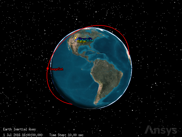
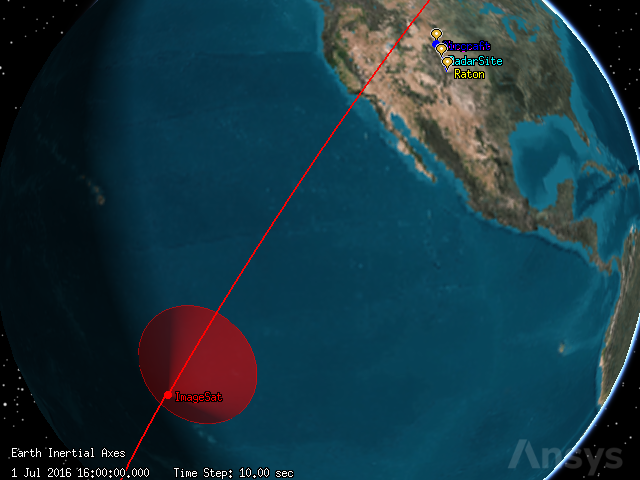
The satellite’s orbit can now be seen in the 3D graphics window:

globe_plotter.show()

Add a fixed sensor on the satellite

The satellite has two sensors. The first sensor is a fixed sensor. A fixed sensor always points in a fixed direction with respect to its parent object. Because this sensor is attached to the satellite, it points with respect to the satellite’s reference frame. And because the satellite is a moving object, even though the sensor is fixed, the sensor’s field-of-view changes along with the satellite’s movement.

The fixed sensor has a simple conic pattern with a \(45^\circ\) cone angle and an angular resolution of \(1^\circ\). Determine if this sensor can see Raton during the analysis period.

First, insert a sensor on the satellite. By default, the sensor’s type is fixed.

fixed_sat_sensor = satellite.children.new(STKObjectType.SENSOR, "FixedSatelliteSensor")

Then, set the sensor’s pattern to simple conic with a cone half angle of \(45^\circ\) and an angular resolution of \(1^\circ\):

from ansys.stk.core.stkobjects import SensorPattern


fixed_sat_sensor.set_pattern_type(SensorPattern.SIMPLE_CONIC)
fixed_sat_sensor.common_tasks.set_pattern_simple_conic(45, 1)

<ansys.stk.core.stkobjects.SensorSimpleConicPattern at 0x701fa87b9400>

It is possible to see the sensor’s field of vision in the 3D graphics window:

globe_plotter.camera.position = [12770, 9060, 4570]
globe_plotter.show()

Compute fixed access

Determine if the fixed sensor on the satellite can take pictures of the site of interest in Raton during the analysis period. To do so, add Raton as an associated object to the sensor. Then, compute access.

Create an access object between the fixed sensor and Raton:

fixed_sat_access = fixed_sat_sensor.get_access_to_object(raton)

Use the access object to compute the accesses between the sensor and Raton:

fixed_sat_access.compute_access()

Then, use the access object’s data providers to get an Access Data report for the time period between the scenario’s start and end times. Convert the report to a pandas data frame for easier viewing:

fixed_sat_access.data_providers.item("Access Data").execute(
    scenario.start_time, scenario.stop_time
).data_sets.to_pandas_dataframe()

	access number	start time	stop time	duration	from pass number	to pass number	from start lat	from start lon	from start alt	from stop lat	...	from stop utm northing	from stop mgrs cell	to start utm zone	to start utm easting	to start utm northing	to start mgrs cell	to stop utm zone	to stop utm easting	to stop utm northing	to stop mgrs cell
0	1	1 Jul 2016 23:18:46.104788812	1 Jul 2016 23:22:28.498370236	222.39358142416313	5	N/A	44.64164650787912	-105.54883102484307	810.5207735074893	34.60088402941391	...	3831.1161866890848	15STU9229331116	13S	549.9610548503704	4084.3031255548854	13SEA4996184303	13S	549.9610548503704	4084.3031255548854	13SEA4996184303
1	2	2 Jul 2016 15:44:40.777714426	2 Jul 2016 15:47:17.087773627	156.31005920104508	15	N/A	37.542558082091475	-114.17830610089635	807.9052096873626	44.50290184962276	...	4929.071566021059	13TCK6804329072	13S	549.9610548503704	4084.3031255548854	13SEA4996184303	13S	549.9610548503704	4084.3031255548854	13SEA4996184303

2 rows × 60 columns

There are two rows in the dataframe, each corresponding to an access. The access durations were approximately 222 and 156 seconds.

Add a moving sensor on a the satellite

Many satellites can gimbal their sensors to track other objects (stationary and moving). STK provides a variety of sensor definitions and pointing types that model this type of movement. In this scenario, the satellite has a second moving sensor targeted towards Raton. Compare the access times for Raton between the fixed and targeted sensors.

First, insert a sensor on the satellite:

moving_sat_sensor = satellite.children.new(
    STKObjectType.SENSOR, "MovingSatelliteSensor"
)

The sensor is inserted as a fixed sensor by default, so set the sensor’s pointing type to targeted:

from ansys.stk.core.stkobjects import SensorPointing


moving_sat_sensor.set_pointing_type(SensorPointing.TARGETED)

Then, set the sensor’s pattern to simple conic with a cone half angle of \(5^\circ\) and an angular resolution of \(1^\circ\):

moving_sat_sensor.set_pattern_type(SensorPattern.SIMPLE_CONIC)
moving_sat_sensor.common_tasks.set_pattern_simple_conic(5, 1)

<ansys.stk.core.stkobjects.SensorSimpleConicPattern at 0x701fa879e0d0>

Because the sensor is set to a pointing type, the sensor’s pointing method now holds an ISensorPointingTargeted object, through which it is possible to add a target to the sensor. Add Raton as the target:

moving_sat_sensor.pointing.targets.add(raton.path)

Compute targeted access

Determine how the access times for the targeted sensor compare to those for the fixed sensor.

First, create an access between the moving sensor and Raton:

moving_sat_access = moving_sat_sensor.get_access_to_object(raton)

Use the access object to compute the accesses between the sensor and Raton:

moving_sat_access.compute_access()

Then, use the access object’s data providers to get an Access Data report for the time period between the scenario’s start and end times and convert the report to a pandas data frame:

moving_sat_access.data_providers.item("Access Data").execute(
    scenario.start_time, scenario.stop_time
).data_sets.to_pandas_dataframe()

	access number	start time	stop time	duration	from pass number	to pass number	from start lat	from start lon	from start alt	from stop lat	...	from stop utm northing	from stop mgrs cell	to start utm zone	to start utm easting	to start utm northing	to start mgrs cell	to stop utm zone	to stop utm easting	to stop utm northing	to stop mgrs cell
0	1	1 Jul 2016 16:06:33.042657963	1 Jul 2016 16:21:57.147955955	924.1052979919818	1	N/A	20.285395880445574	-129.36567072017962	802.5561749123867	58.16691058496301	...	6450.592739939335	18VUK3822250593	13S	549.9610548503704	4084.3031255548854	13SEA4996184303	13S	549.9610548503704	4084.3031255548854	13SEA4996184303
1	2	1 Jul 2016 17:54:25.049202786	1 Jul 2016 18:06:09.202906987	704.153704200563	2	N/A	40.53911501672179	-139.47747693234007	808.9972819417733	60.11255386714036	...	6663.97327721914	17VMG8588763973	13S	549.9610548503704	4084.3031255548854	13SEA4996184303	13S	549.9610548503704	4084.3031255548854	13SEA4996184303
2	3	1 Jul 2016 19:43:08.544272897	1 Jul 2016 19:52:18.284449259	549.7401763618254	3	N/A	57.46958434196302	-132.12912969952245	815.170217000789	55.027558199500405	...	6098.329936014981	18UWF6494598330	13S	549.9610548503704	4084.3031255548854	13SEA4996184303	13S	549.9610548503704	4084.3031255548854	13SEA4996184303
3	4	1 Jul 2016 21:28:32.969348323	1 Jul 2016 21:41:19.325132041	766.3557837182198	4	N/A	60.01071454326304	-127.84047347095935	816.0143210664654	35.392058818758194	...	3917.4431020001534	19SCV7137817443	13S	549.9610548503704	4084.3031255548854	13SEA4996184303	13S	549.9610548503704	4084.3031255548854	13SEA4996184303
4	5	1 Jul 2016 23:12:41.028600008	1 Jul 2016 23:28:27.709287771	946.6806877629606	5	N/A	57.193943265114484	-132.49532888485777	815.0764267012754	16.826005531878987	...	1861.8988647264814	17QKU4091661899	13S	549.9610548503704	4084.3031255548854	13SEA4996184303	13S	549.9610548503704	4084.3031255548854	13SEA4996184303
5	6	2 Jul 2016 00:57:36.720961000	2 Jul 2016 01:11:41.846264778	845.125303777364	6	N/A	49.55412901747986	-138.36276507628673	812.3481178216941	9.558456673642443	...	1056.595898644507	13PDL8986856596	13S	549.9610548503704	4084.3031255548854	13SEA4996184303	13S	549.9610548503704	4084.3031255548854	13SEA4996184303
6	7	2 Jul 2016 13:54:26.287176229	2 Jul 2016 14:09:07.045792985	880.7586167559202	14	N/A	9.642605023436763	-106.89201070734224	800.5985462954347	50.94108778443152	...	5645.431433369973	19UCS5044445431	13S	549.9610548503704	4084.3031255548854	13SEA4996184303	13S	549.9610548503704	4084.3031255548854	13SEA4996184303
7	8	2 Jul 2016 15:38:13.754078366	2 Jul 2016 15:53:50.037053064	936.2829746974894	15	N/A	18.60479861000556	-127.59844985434151	802.164758225905	57.743833777263376	...	6402.183831738761	18VUK7322702184	13S	549.9610548503704	4084.3031255548854	13SEA4996184303	13S	549.9610548503704	4084.3031255548854	13SEA4996184303

8 rows × 60 columns

The targeted sensor is able to access Raton 8 times, as opposed to the fixed sensor’s 2 accesses. The targeted sensor’s accesses are also longer, ranging between approximately 549 and 946 seconds. The increased access is because the targeted sensor locks onto the assigned target using the sensor’s boresight. This represents point-to-point access. Because the access is only constrained by the line-of-site, the targeted sensor can access Raton from horizon to horizon. The field of view of the fixed sensor has to pass over Raton to be able to access it, so the access time for the targeted sensor is much higher.

Conclusion: Both cameras attached to the imaging satellite have opportunities to take pictures of Raton.

Add a fixed sensor on the radar site

Now, determine if the radar site can see an aircraft flying between Cheyenne and Raton. The site has two sensors, one of which is a fixed sensor. Sensors can be used to model instruments attached to stationary objects, such as Facility, Place, and Target objects. Fixed sensors attached to stationary objects also point with respect to the parent object’s reference frame. Since stationary objects never change position or direction, a fixed sensor on a fixed object always points in a fixed direction. The radar site has one fixed sensor representing the site’s entire possible field of view.

First, add a sensor to the radar site. The sensor is inserted as a fixed sensor by default.

radar_dome_sensor = radar_site.children.new(STKObjectType.SENSOR, "RadarDome")

Then, set the sensor’s pattern to simple conic with a cone half angle of \(90^\circ\) and an angular resolution of \(1^\circ\):

radar_dome_sensor.set_pattern_type(SensorPattern.SIMPLE_CONIC)
radar_dome_sensor.common_tasks.set_pattern_simple_conic(90, 1)

<ansys.stk.core.stkobjects.SensorSimpleConicPattern at 0x701f05362ad0>

Add a constraint to the sensor

The fixed sensor attached to the facility is similar to the fixed sensor attached to the imaging satellite. However, the site’s sensor has a larger field-of-view, and instead of pointing straight down this sensor points straight up from the radar site. So, the sensor has an upwards looking field-of-view that covers everything above the site. This is not a realistic field of view, so limit the sensor’s range so that the field-of-view spans a constrained area mimicking the field-of-view of the actual air traffic control radar. Limit the field-of-view to a maximum range of \(150\) km.

First, add a range access constraint to the sensor:

from ansys.stk.core.stkobjects import AccessConstraintType


dome_range_constraint = radar_dome_sensor.access_constraints.add_constraint(
    AccessConstraintType.RANGE
)

Then, set the constraint to have a maximum range of \(150\) km:

dome_range_constraint.enable_maximum = True
dome_range_constraint.maximum = 150

The sensor can now only see \(150\) km in each direction.

Configure the 2D projection properties

2D graphics projection properties for sensors control the display of sensor projection graphics in the 2D Graphics window. When the sensor’s display is set to project to the range constraint, STK projects the sensor’s field-of-view to the maximum range previously specified for the sensor.

Configure the sensor’s 2D graphics properties to show a projection of the maximum range on the 2D map:

from ansys.stk.core.stkobjects import SensorProjectionDistanceType


radar_dome_sensor.graphics.projection.distance_type = (
    SensorProjectionDistanceType.RANGE_CONSTRAINT
)
radar_dome_sensor.graphics.projection.use_constraints = True
radar_dome_sensor.graphics.projection.show_on_2d_map = True

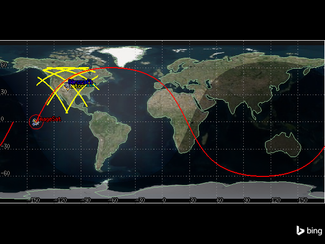
It is now possible to see the range of \(150\) km around the radar site on the 2D graphics window:

map_plotter.show()

Calculate access

From the projection on the map, it is clear that the fixed sensor can access the flight along its route. Now, determine how long the sensor can access the flight for.

Create an access between the sensor and the aircraft:

radar_dome_access = radar_dome_sensor.get_access_to_object(aircraft)

Compute the accesses between the sensor and aircraft:

radar_dome_access.compute_access()

View the Access Data report for the scenario’s duration as a pandas dataframe:

radar_dome_access_df = (
    radar_dome_access.data_providers.item("Access Data")
    .execute(scenario.start_time, scenario.stop_time)
    .data_sets.to_pandas_dataframe()
)

radar_dome_access_df

	access number	start time	stop time	duration	from pass number	to pass number	from start lat	from start lon	from start alt	from stop lat	...	from stop utm northing	from stop mgrs cell	to start utm zone	to start utm easting	to start utm northing	to start mgrs cell	to stop utm zone	to stop utm easting	to stop utm northing	to stop mgrs cell
0	1	1 Jul 2016 16:29:43.607470276	1 Jul 2016 17:22:37.021112289	3173.4136420134782	N/A	N/A	38.800599999999996	-104.6784	1.8668522680687163	38.800599999999996	...	4294.698440149648	13SEC2792694698	13S	525.2803264091833	4417.176131815217	13SEE2528017176	13S	543.3820054180567	4173.1739066086	13SEB4338273174

1 rows × 60 columns

The fixed sensor can view the aircraft for approximately \(3173\) seconds.

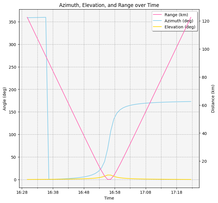
Generate an AER report

An AER (azimuth, elevation, and range) report describes the location of the aircraft when it is within the sensor’s view. This data can be useful for many purposes, including air traffic control. To get the AER report, first select the AER Data report from the access’s data providers. Then, select the Default report from the IDataProviders object stored in the IDataProviderGroup’s group property. Finally, convert the report to a pandas dataframe:

aer_df = (
    radar_dome_access.data_providers.item("AER Data")
    .group.item("Default")
    .execute(scenario.start_time, scenario.stop_time, 60)
    .data_sets.to_pandas_dataframe()
)

It is now possible to graph the azimuth, elevation, and range data:

import matplotlib.dates as md
import matplotlib.pyplot as plt
import pandas as pd


# Convert columns to correct types
aer_df["time"] = pd.to_datetime(aer_df["time"])
aer_df.set_index("time", inplace=True)
cols = ["azimuth", "elevation", "range"]
aer_df[cols] = aer_df[cols].apply(pd.to_numeric)

# Create a plot and duplicate the x-axis
fig, ax1 = plt.subplots(figsize=(8, 8))
ax2 = ax1.twinx()

# Plot range, azimuth, and elevation
(line1,) = ax2.plot(aer_df.index, aer_df["range"], color="hotpink", label="Range (km)")
(line2,) = ax1.plot(
    aer_df.index, aer_df["azimuth"], color="skyblue", label="Azimuth (deg)"
)
(line3,) = ax1.plot(
    aer_df.index, aer_df["elevation"], color="gold", label="Elevation (deg)"
)

# Set title and axes labels
ax1.set_title("Azimuth, Elevation, and Range over Time")
ax1.set_xlabel("Time")
ax1.set_ylabel("Angle (deg)")
ax2.set_ylabel("Distance (km)")

# Combine legends
lines = [line1, line2, line3]
labels = [line.get_label() for line in lines]
ax1.legend(lines, labels, shadow=True)

# Configure style
ax1.set_facecolor("whitesmoke")
ax1.grid(visible=True, which="both", linestyle="--")

# Improve x-axis formatting
formatter = md.DateFormatter("%H:%M")
ax1.xaxis.set_major_formatter(formatter)
# Set major and minor locators
xlocator_major = md.MinuteLocator(interval=10)
xlocator_minor = md.MinuteLocator(interval=5)
ax1.xaxis.set_major_locator(xlocator_major)
ax1.xaxis.set_minor_locator(xlocator_minor)
plt.show()

Add a moving sensor to the control site

Often, the dome created by a fixed sensor object is used to model a field-of-view, or the overall volume of space in which radar looks. The radar itself often sweeps or scans through that field-of-view in a repeating cycle. The area of space represented by such a scanning or spinning radar at any given instant is its field-of-view. To model the aircraft control site’s radar itself, build a sweeping radar beam using a moving sensor.

First, insert a sensor on the radar site:

radar_sweep_sensor = radar_site.children.new(STKObjectType.SENSOR, "RadarSweep")

To model a field-of-view of a radar, use a rectangular sensor. Rectangular sensor types are typically used for modeling the field-of-view of instruments such as push broom sensors and star trackers. Rectangular sensors are defined according to specified vertical and horizontal half-angles.

Set the radar’s sensor pattern to a rectangular pattern with a \(5^\circ\) vertical half angle and a \(35^\circ\) horizontal half angle:

radar_sweep_sensor.set_pattern_type(SensorPattern.RECTANGULAR)
radar_sweep_sensor.common_tasks.set_pattern_rectangular(5, 35)

<ansys.stk.core.stkobjects.SensorRectangularPattern at 0x701f04b5aba0>

This sensor configuration creates a wedge type field-of-view. Right now, that “wedge” is just pointing straight up. The radar afixed to the radar site sweeps or scans in a repeating cycle. Since the radar “scans”, the full range of the radar is not always covered. Configure the sensor’s field-of-view to provide a visual representation of the area that the radar does cover at any given point in time. Set the properties of the sensor to rotate and point at \(35^\circ\) elevation. Set the spin axis elevation to \(90^\circ\) for horizontal rotation with a cone angle of \(55^\circ\) for a \(35^\circ\) elevation from the horizon.

First, set the radar’s pointing type to spinning. This type of sensor is used to model radars, push broom sensors, and other instruments that spin, scan, or sweep over time.

radar_sweep_sensor.set_pointing_type(SensorPointing.SPINNING)

The sensor’s pointing property now contains an ISensorPointingSpinning object. The spin rate property of this object describes the rate at which the boresight spins about the spin axis, measured in revolutions per minute. Set the spin rate to \(12\) revs/min:

radar_sweep_sensor.pointing.spin_rate = 12

The spin axis cone angle of the object designates the cone angle used in defining the spin axis, i.e. the angle between the spin axis and the sensor boresight. Set the spin axis cone angle to \(55^\circ\):

radar_sweep_sensor.pointing.spin_axis_cone_angle = 55

Add a constraint to the sensor

Right now, the field-of-view extends beyond the limits of the actual radar (modeled with the fixed sensor) because there are no constraints on the moving sensor. The airport’s primary surveillance radar has a range of \(150\) km, so limit the range of the moving sensor to model that constraint.

First, add a range constraint to the sweeping sensor:

sweep_range_constraint = radar_sweep_sensor.access_constraints.add_constraint(
    AccessConstraintType.RANGE
)

Then, configure the constraint to a maximum range of \(150\) km:

sweep_range_constraint.enable_maximum = True
sweep_range_constraint.maximum = 150

Configure the 2D projection properties

To view the moving sensor’s field of view on the 2D graphics window, configure some of the sensors graphics properties:

from ansys.stk.core.utilities.colors import Color


radar_sweep_sensor.graphics.projection.distance_type = (
    SensorProjectionDistanceType.RANGE_CONSTRAINT
)
radar_sweep_sensor.graphics.projection.use_constraints = True
radar_sweep_sensor.graphics.projection.show_on_2d_map = True
radar_sweep_sensor.graphics.color = Color.from_rgb(247, 57, 57)
radar_dome_sensor.graphics.color = Color.from_rgb(199, 247, 87)

The sweeping radar’s field-of-view can now be seen in red, while the fixed sensor’s field-of-view is seen in yellow:

map_plotter.show()

Calculate access

Now, determine when the sweeping radar sensor can see the aircraft flying between Cheyenne and Raton. To do so, first create an access between the sensor and the aircraft:

sweeping_access = radar_sweep_sensor.get_access_to_object(aircraft)

Then, compute the access:

sweeping_access.compute_access()

View the Access Data report as a pandas dataframe:

sweeping_access_df = (
    sweeping_access.data_providers.item("Access Data")
    .execute(scenario.start_time, scenario.stop_time)
    .data_sets.to_pandas_dataframe()
)

sweeping_access_df

	access number	start time	stop time	duration	from pass number	to pass number	from start lat	from start lon	from start alt	from stop lat	...	from stop utm northing	from stop mgrs cell	to start utm zone	to start utm easting	to start utm northing	to start mgrs cell	to stop utm zone	to stop utm easting	to stop utm northing	to stop mgrs cell
0	1	1 Jul 2016 16:29:44.958476865	1 Jul 2016 16:29:45.067448532	0.10897166734162056	N/A	N/A	38.800599999999996	-104.6784	1.8668522680687163	38.800599999999996	...	4294.698440149648	13SEC2792694698	13S	525.2880419880917	4417.072255649128	13SEE2528817072	13S	525.2886643234249	4417.063877037749	13SEE2528917064
1	2	1 Jul 2016 16:29:49.957308016	1 Jul 2016 16:29:50.070742561	0.11343454465827563	N/A	N/A	38.800599999999996	-104.6784	1.8668522680687163	38.800599999999996	...	4294.698440149648	13SEC2792694698	13S	525.3165901863425	4416.687905600609	13SEE2531716688	13S	525.3172380071794	4416.679183846731	13SEE2531716679
2	3	1 Jul 2016 16:29:54.958698843	1 Jul 2016 16:29:55.068800787	0.11010194458481237	N/A	N/A	38.800599999999996	-104.6784	1.8668522680687163	38.800599999999996	...	4294.698440149648	13SEC2792694698	13S	525.3451529184847	4416.303358705142	13SEE2534516303	13S	525.3457817050986	4416.294893187323	13SEE2534616295
3	4	1 Jul 2016 16:29:59.959716422	1 Jul 2016 16:30:00.070418384	0.11070196206992478	N/A	N/A	38.800599999999996	-104.6784	1.8668522680687163	38.800599999999996	...	4294.698440149648	13SEC2792694698	13S	525.3737134345658	4415.918840469133	13SEE2537415919	13S	525.3743456459795	4415.910328816316	13SEE2537415910
4	5	1 Jul 2016 16:30:04.959121338	1 Jul 2016 16:30:05.069712012	0.11059067382325338	N/A	N/A	38.800599999999996	-104.6784	1.8668522680687163	38.800599999999996	...	4294.698440149648	13SEC2792694698	13S	525.4022646563006	4415.534446188857	13SEE2540215534	13S	525.4028962302825	4415.525943091916	13SEE2540315526
...	...	...	...	...	...	...	...	...	...	...	...	...	...	...	...	...	...	...	...	...	...
630	631	1 Jul 2016 17:22:12.542211189	1 Jul 2016 17:22:12.655395658	0.11318446960285655	N/A	N/A	38.800599999999996	-104.6784	1.8668522680687163	38.800599999999996	...	4294.698440149648	13SEC2792694698	13S	543.2425746033616	4175.056097742356	13SEB4324375056	13S	543.2432193057092	4175.047394952162	13SEB4324375047
631	632	1 Jul 2016 17:22:17.542592419	1 Jul 2016 17:22:17.655082448	0.11249002877684688	N/A	N/A	38.800599999999996	-104.6784	1.8668522680687163	38.800599999999996	...	4294.698440149648	13SEC2792694698	13S	543.2710568611676	4174.671616801334	13SEB4327174672	13S	543.2716976045938	4174.662967405843	13SEB4327274663
632	633	1 Jul 2016 17:22:22.543656683	1 Jul 2016 17:22:22.654072502	0.1104158197513243	N/A	N/A	38.800599999999996	-104.6784	1.8668522680687163	38.800599999999996	...	4294.698440149648	13SEC2792694698	13S	543.2995428597874	4174.287083293751	13SEB4330074287	13S	543.3001717852065	4174.278593383817	13SEB4330074279
633	634	1 Jul 2016 17:22:27.543506275	1 Jul 2016 17:22:27.653337854	0.10983157959071832	N/A	N/A	38.800599999999996	-104.6784	1.8668522680687163	38.800599999999996	...	4294.698440149648	13SEC2792694698	13S	543.3280217898402	4173.90264313468	13SEB4332873903	13S	543.328647384151	4173.894198146116	13SEB4332973894
634	635	1 Jul 2016 17:22:32.542642434	1 Jul 2016 17:22:32.652370697	0.10972826379656908	N/A	N/A	38.800599999999996	-104.6784	1.8668522680687163	38.800599999999996	...	4294.698440149648	13SEC2792694698	13S	543.3564965063458	4173.51825778372	13SEB4335673518	13S	543.3571215088847	4173.509820738092	13SEB4335773510

635 rows × 60 columns

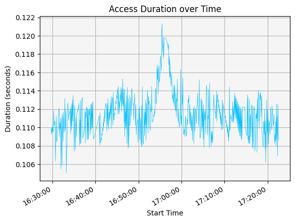
The sweeping radar is able to access the aircraft 635 times during the aircraft’s flight, as indicated by the 635 rows in the dataframe.

Now, use the dataframe to convert the duration column to numeric form and calculate the average duration of access between the sensor and the aircraft:

import pandas as pd


sweeping_access_df["duration"] = pd.to_numeric(sweeping_access_df["duration"])
sweeping_access_df.mean(numeric_only=True)["duration"]

np.float64(0.11156903697293434)

The average duration of access was approximately \(0.111\) seconds.

Visualize access with a graph

The duration and time of access can be visualized with a graph.

import matplotlib.dates as md


# Convert data to correct type
sweeping_access_df["start time"] = pd.to_datetime(sweeping_access_df["start time"])

# Plot data
ax = sweeping_access_df.plot(
    x="start time", y="duration", color="deepskyblue", linewidth=0.5
)

# Set title and axes labels
ax.set_title("Access Duration over Time")
ax.set_xlabel("Start Time")
ax.set_ylabel("Duration (seconds)")

# Configure the style of the plot
ax.get_legend().remove()
ax.set_facecolor("whitesmoke")
ax.grid(visible=True, which="both")

# Improve x-axis formatting
formatter = md.DateFormatter("%H:%M:%S")
ax.xaxis.set_major_formatter(formatter)

plt.show()

Analyze multiple accesses

Create an access graph that shows all four sensors and their accesses to the aircraft. There are already existing calculations in this scenario for the access between the radar site’s fixed and moving sensors and the aircraft. However, there are no access calculations between either of the sensors on the satellite and the aircraft.

First, create an access between the satellite’s fixed sensor and the aircraft:

fixed_aircraft_access = fixed_sat_sensor.get_access_to_object(aircraft)

Then, compute the access:

fixed_aircraft_access.compute_access()

Convert the “Access Duration” report to a pandas dataframe:

fixed_aircraft_access_df = (
    fixed_aircraft_access.data_providers.item("Access Data")
    .execute(scenario.start_time, scenario.stop_time)
    .data_sets.to_pandas_dataframe()
)

Then, create an access between the satellite’s moving sensor and the aircraft:

moving_aircraft_access = moving_sat_sensor.get_access_to_object(aircraft)

Then, compute the access:

moving_aircraft_access.compute_access()

Finally, convert the “Access Duration” report to a pandas dataframe:

moving_aircraft_access_df = (
    moving_aircraft_access.data_providers.item("Access Data")
    .execute(scenario.start_time, scenario.stop_time)
    .data_sets.to_pandas_dataframe()
)

Now, there are access duration reports for the accesses between all four sensors in the scenario and the aircraft. Group these reports into a list:

access_reports = [
    fixed_aircraft_access_df,
    moving_aircraft_access_df,
    sweeping_access_df,
    radar_dome_access_df,
]

Convert the start and stop times for each report to a time format, and the duration columns to a time delta format:

for report in access_reports:
    report["start time"] = pd.to_datetime(report["start time"])
    report["stop time"] = pd.to_datetime(report["stop time"])
    report["duration"] = pd.to_numeric(report["duration"])
    report["duration"] = pd.to_timedelta(report["duration"], unit="seconds")

Then, graph all the reports together in an event plot:

import datetime as dt


# Create plot
fig, ax = plt.subplots()
ax.broken_barh(
    list(
        zip(
            fixed_aircraft_access_df["start time"], fixed_aircraft_access_df["duration"]
        )
    ),
    (10, 9),
    facecolors="cornflowerblue",
    label="Fixed sensor on satellite",
)
ax.broken_barh(
    list(
        zip(
            moving_aircraft_access_df["start time"],
            moving_aircraft_access_df["duration"],
        )
    ),
    (20, 9),
    facecolors="aquamarine",
    label="Moving sensor on satellite",
)
ax.broken_barh(
    list(zip(sweeping_access_df["start time"], sweeping_access_df["duration"])),
    (30, 9),
    facecolors="mediumslateblue",
    label="Sweeping radar",
)
ax.broken_barh(
    list(zip(radar_dome_access_df["start time"], radar_dome_access_df["duration"])),
    (40, 9),
    facecolors="lightpink",
    label="Fixed radar dome",
)

# Set title and axes labels
ax.set_title("Access To Aircraft by Sensor")
ax.set_xlabel("Time")
ax.get_yaxis().set_visible(False)

# Configure the style of the plot
ax.legend()
ax.set_facecolor("whitesmoke")

# Set the size of the plot
fig.set_size_inches(16, 5)

# Improve x-axis formatting
formatter = md.DateFormatter("%H:%M:%S")
ax.xaxis.set_major_formatter(formatter)
ax.minorticks_on()

plt.show()

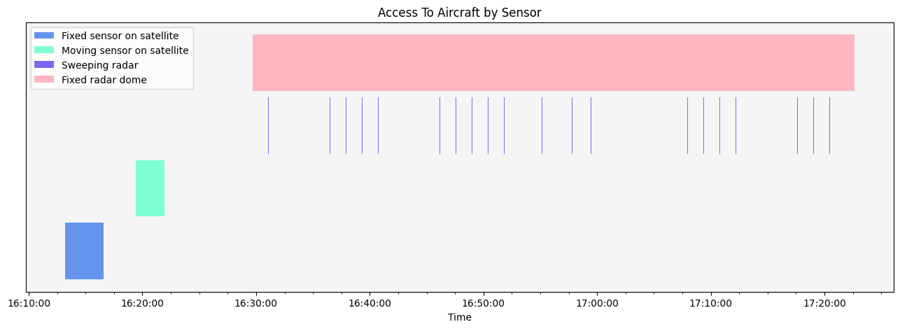
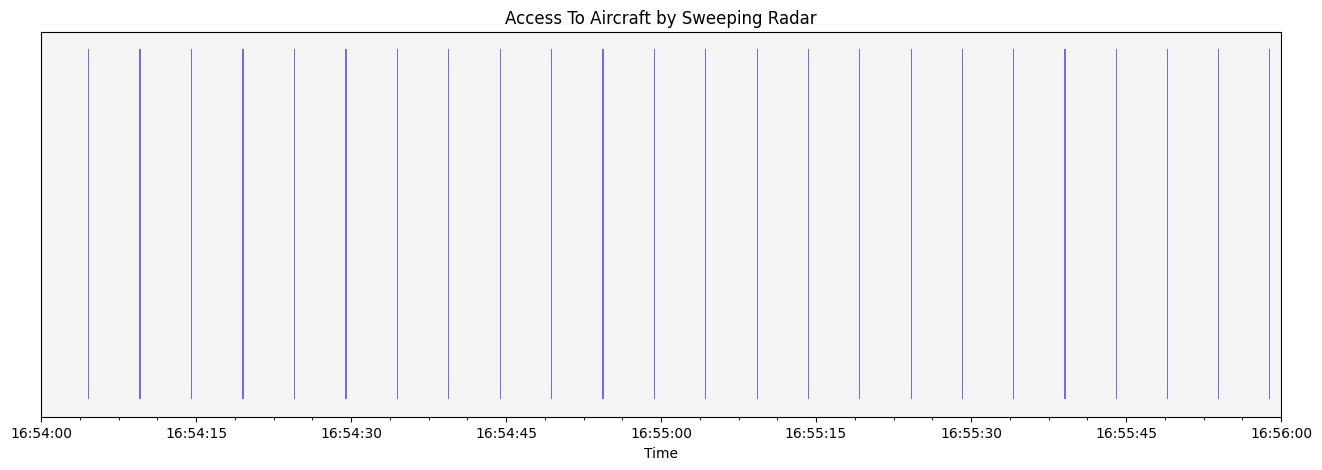
The graph shows that all of the sensors can see the aircraft during its flight, with the fixed radar dome able to see the aircraft for the longest duration of time. However, because the sweeping radar sees the aircraft for very short bursts of time, it is difficult to make out the different accesses. To better see the sweeping radar’s accesses, create a plot zoomed in on the access between 16:54 and 16:56.

# Create plot
fig, ax = plt.subplots()
ax.broken_barh(
    list(zip(sweeping_access_df["start time"], sweeping_access_df["duration"])),
    (30, 9),
    facecolors="mediumslateblue",
    label="Sweeping radar",
)

# Set title and axes labels
ax.set_title("Access To Aircraft by Sweeping Radar")
ax.set_xlabel("Time")
ax.get_yaxis().set_visible(False)

# Configure the style of the plot
ax.set_facecolor("whitesmoke")

# Set the size of the plot
fig.set_size_inches(16, 5)

# Improve x-axis formatting
formatter = md.DateFormatter("%H:%M:%S")
ax.xaxis.set_major_formatter(formatter)
ax.minorticks_on()
ax.set_xlim(
    left=dt.datetime(2016, 7, 1, 16, 54, 0), right=dt.datetime(2016, 7, 1, 16, 56, 0)
)

plt.show()

Conclusion: All of the sensors involved in the scenario can see the aircraft during its flight.